Universal Radio Hacker: Investigate Wireless Protocols like a Boss

This article is from Open Source Tools edition, that you can download for free if you have an account on our website.

Refers to URH version: 1.9.1

Contact:

1	Introduction
	1.1	Motivation . . . . . . . . . . . . . . . . . . . . . . . . . . . . . . . . . . . . . . . . .
	1.2	Installation . . . . . . . . . . . . . . . . . . . . . . . . . . . . . . . . . . . . . . . . .
2	Device interaction
	2.1	Configuring Devices . . . . . . . . . . . . . . . . . . . . . . . . . . . . . . . . . . .
		2.1.1	Native Backend . . . . . . . . . . . . . . . . . . . . . . . . . . . . . . . . . .
		2.1.2	GNU Radio Backend . . . . . . . . . . . . . . . . . . . . . . . . . . . . . .
	2.2	Scanning the spectrum . . . . . . . . . . . . . . . . . . . . . . . . . . . . . . . .
	2.3	Recording a signal . . . . . . . . . . . . . . . . . . . . . . . . . . . . . . . . . . . .
3	Interpretation
	3.1	Importing a signal . . . . . . . . . . . . . . . . . . . . . . . . . . . . . . . . . . . .
	3.2	Signal editing . . . . . . . . . . . . . . . . . . . . . . . . . . . . . . . . . . . . . . .
	3.3	Replay signal and view signal details . . . . . . . . . . . . . . . . . . . . .
	3.4	Demodulation . . . . . . . . . . . . . . . . . . . . . . . . . . . . . . . . . . . . . . .
	3.5	Spectrogram . . . . . . . . . . . . . . . . . . . . . . . . . . . . . . . . . . . . . . . .
	3.6	Filters (advanced feature) . . . . . . . . . . . . . . . . . . . . . . . . . . . . . .
		3.6.1	Bandpass filter . . . . . . . . . . . . . . . . . . . . . . . . . . . . . . . . . .
		3.6.2	Moving average filter . . . . . . . . . . . . . . . . . . . . . . . . . . . . .
4	Analysis
	4.1	Getting data into analysis . . . . . . . . . . . . . . . . . . . . . . . . . . . . . .
	4.2	Project files . . . . . . . . . . . . . . . . . . . . . . . . . . . . . . . . . . . . . . . . .
	4.3	View data from different perspectives . . . . . . . . . . . . . . . . . . .
	4.4	Decoding . . . . . . . . . . . . . . . . . . . . . . . . . . . . . . . . . . . . . . . . . .
		4.4.1	Configure Decodings . . . . . . . . . . . . . . . . . . . . . . . . . . . . .
		4.4.2	External Decodings . . . . . . . . . . . . . . . . . . . . . . . . . . . . . . .
		4.4.3	Choose decoding . . . . . . . . . . . . . . . . . . . . . . . . . . . . . . . . .
	4.5	Participants . . . . . . . . . . . . . . . . . . . . . . . . . . . . . . . . . . . . . . . .
	4.6		Labs. . . . . . . . . . . . . . . . . . . . . . . . . . . . . . . . . . . . . . . . . . . .
		4.6.1	Assigning and editing labels . . . . . . . . . . . . . . . . . . . . . . . .
		4.6.2	Field Types . . . . . . . . . . . . . . . . . . . . . . . . . . . . . . . . . . . .
		4.6.3	Checksum labels . . . . . . . . . . . . . . . . . . . . . . . . . . . . . . . . .
	4.7	Message Types . . . . . . . . . . . . . . . . . . . . . . . . . . . . . . . . . . . . . . .
5	Generation
	5.1	Fuzzing . . . . . . . . . . . . . . . . . . . . . . . . . . . . . . . . . . . . . . . . . . .
	5.2	Modulation . . . . . . . . . . . . . . . . . . . . . . . . . . . . . . . . . . . . . . . . .
	5.3	Sending it back . . . . . . . . . . . . . . . . . . . . . . . . . . . . . . . . . . . . . .
6	Configuring Look and Feel
7	Plugins

1 Introduction

1.1 Motivation

The Universal Radio Hacker (URH) is a tool for analyzing unknown wireless protocols. With the rise of Internet of Things (IoT) such protocols often appear in the wild. Many IoT devices operate on frequencies like 433.92 MHz or 868.3 MHz and use proprietary protocols for communication. Reverse-engineering such protocols can be fascinating (»What does my fridge talk about?«) and reveal serious security leaks, e.g. when bypassing smart alarm systems and door locks.

So how can we join this game? Software Defined Radios (SDR) are the answer for this. Such devices allow sending and receiving on nearly arbitrary frequencies. Figure 1 shows two examples. Both devices cost about 200 euro

(a) HackRF One can send and receive on frequencies from 1 MHz to 6 GHz. (b) SDRplay RSP2pro can receive on frequencies from 1 kHz to 2 GHz.

Figure 1: Two examples for Software Defined Radios.

Like the name suggests, SDRs need software to be properly operated. This is where the Universal Radio Hacker comes into play: It takes the samples from the SDR and transforms them into binary information (bits). But this is only the beginning: URH is designed to help you throughout the entire process of attacking the wireless communication of IoT devices. In the upcoming sections, you will learn how to use URH and reverse engineer wireless protocols in minutes.

1.2 Installation

URH runs on Linux, OSX and Windows and is easy to install. You can nd the latest installation instructions here: https://github.com/jopohl/urh#installation

2 Device interaction

To get started with investigating a wireless signal we need to capture it with a Software Defined Radio. URH offers support for a wide range of common SDRs. In this section, you will learn how to configure your SDR and use it inside URH.

2.1 Configuring Devices

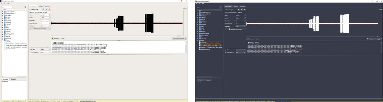
First, let's ensure that your device is enabled in Edit Options Device. You will see a list of supported devices, similar to what is shown in fig. 2a.

(a) Device options tab. (b) Health check native backend.

Figure 2: Configuring devices

If you select a device in the list, you can either enable/disable it via the Enabled checkbox. Disabling a device will prevent it from showing up in the device selection in the main program. Furthermore, you can choose between native and GNU Radio backend. More on this in the following sections.

2.1.1 Native Backend

The native device backend should be used whenever possible. If native backend is greyed out for a device, there may be a library missing. You can check this by clicking the Health Check button. A dialog like the one shown in fig. 2b will pop up and give you more information about the status of native device backend. If you indeed miss a library, you can install it on your system. For example, install HackRF library on Ubuntu with sudo apt-get install libhackrf-dev. After that, hit the Rebuild button at the bottom of the dialog.

2.1.2 GNU Radio Backend

As a fallback to the native backend, you can use GNU Radio to access your device. In order to do that, configure either the path to your Python 2 interpreter or (on Windows) the GNU Radio installation directory. Then, you get notified that GNU Radio backend is available and can choose it after selecting your desired device from the device list in fig. 2a.

2.2 Scanning the spectrum

Having configured our SDR, let’s start by scanning the wireless spectrum and find the center frequency of the device we want to attack. To open the spectrum analyzer, use File → Spectrum Analyzer, this will give you a dialog as shown in section 2.2.

Figure 3: Spectrum Analyzer dialog.

Device settings can be made on the left. After starting the spectrum analyzer, you can watch how URH tunes your device to the desired parameters in the bottom left.

When spectrum analysis starts, you see the spectrum at the top right and a waterfall plot of the spectrum in the bottom right. Both views together give you a good impression of the spectrum and allow you to find the target frequency easily. To change the current frequency you can either use the spinbox on the left or click on the desired point in the spectrum. This way, you can navigate through the spectrum and visually find the desired frequency.

2.3 Recording a signal

Having found the target frequency, it is time to record a signal for later analysis. Open up the recording dialog via File→Record Signal and you will see that it saved your parameters from Spectrum Analyzer, so you can simply start the recording with the record button on the middle left. In fig. 4 recording is already running and a wireless remote control was pressed two times. You can clearly see the two signals in the preview on the right.

Figure 4: Record signals in this dialog

Stop the recording with the stop button. After this, you can save the signal and make another recording or simply close the dialog. You will be asked if you want to save your current recording. Congratulations, you successfully recorded your first signal!

3 Interpretation

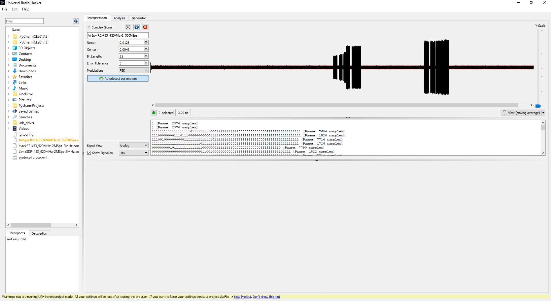
Having recorded a signal, URH adds it automatically to the Interpretation Tab (fig. 5). Before we explore this tab, let’s have a look at other ways of opening and importing a signal.

3.1 Importing a signal

Apart from recording, a signal can be added to Interpretation tab via File →Open. File ending determines how URH handles the signal. URH understands these file endings:

.complex files with complex64 samples (32 Bit oat for I and Q, respectively). This is the default signal file format and will also be used in case the le has no ending at all.
.complex16u using two unsigned 8 Bit integers for I and Q
.complex16s using two signed 8 Bit integers for I and Q
.wav files can be imported, but must not be compressed, i.e., they should be PCM.
.csv, e.g. from USB oscilloscope can be imported using a CSV wizard available with File →Import→ IQ samples from csv.

3.2 Signal editing

Having loaded a signal into Interpretation, it can be zoomed using the mouse wheel or context menu. Make a selection with the mouse and navigate via drag by holding the shift key. This can be changed with the checkbox Edit →Options→ Hold shift to drag.

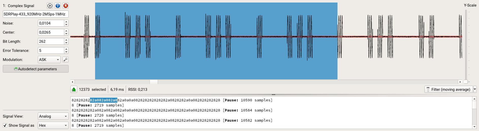
Figure 5: Recorded signal gets automatically added to Interpretation tab.

Apart from these basic functions, URH has a powerful signal editor. After making a selection, use the context menu to:

Copy/paste parts of the signal
Delete the selection
Crop to current selection, i.e., remove everything that is not selected

- Mute the selection, i.e., set the selected part to zero
- Create a new signal from the selection
- Assign a participant more on this in section 4.5
Set noise level from selection

Using these features you can isolate interesting signal parts and fix noisy recordings.

3.3 Replay signal and view signal details

With the button in the top of fig. 5 you can replay the captured signal. Thebutton opens signal detail dialog (fig. 6) where you can also edit the sample rate. This influences the displayed time in Interpretation and Analysis.

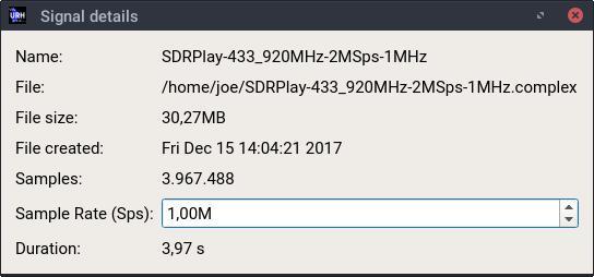
Figure 6: Signal detail dialog.

3.4 Demodulation

Demodulation is the process of converting the recorded sine waves into bits. URH does this automatically for you whenever you add a signal to Interpretation tab. You see the resulting bits right below the signal.

You can change the modulation type using the combobox on the left. Whenever you change the modulation type the demodulation parameters are newly detected by URH. You can disable this by clicking the Autodetect parameters button. Of course, you can fine tune the parameters by using the spinboxes.

The demodulation parameters are:

Noise: Define which power must be surpassed to not be counted as noise.
Bit Length: The sample length of a bit. You can find this out by selecting a pulse with minimum length and looking at the number of selected samples as shown in fig. 7a.
Center: The center in demodulated view separates the ones from the zeros. To tune this value, either use the spinbox or change the Signal View from Analog to Demodulated (see fig. 7b) and move the center between the areas with the mouse.
Error Tolerance: Fine tune how tolerant (in samples) the demodulation routine shall be against errors.

Note that these parameters are found automatically and only need to be changed manually in rare cases, e.g. bad signal recordings.

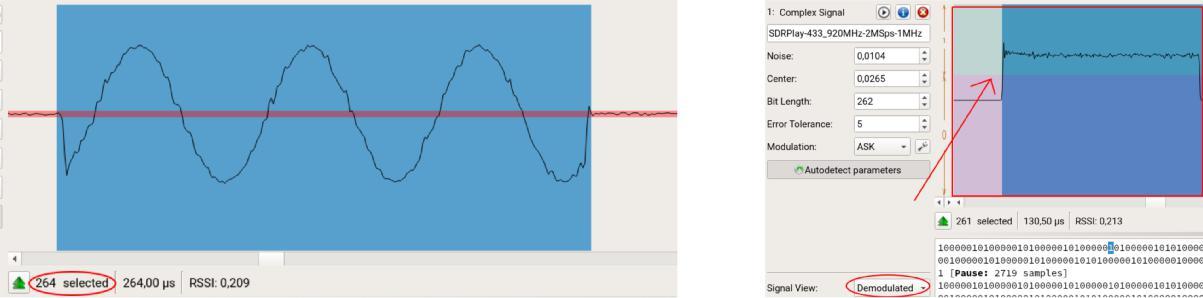
(a) Finding the bit length manually. (b) Setting the center for demodulation.

Figure 7: Finding bit length and center visually.

In case of ASK demodulation, you can make advanced settings using the button next to the demodulation combobox.

3.5 Spectrogram

With the spectrogram view (fig. 8), you can view the frequency spectrum of your signal during time. Simply switch to this view via Signal View→ Spectrogram.

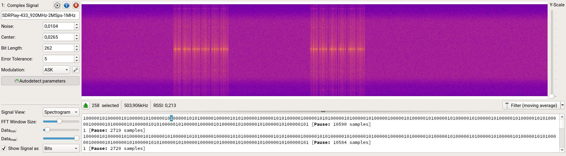
Figure 8: Spectrogram view for a signal.

The spectrogram view has three parameters:

FFT Window Size is the used STFT (Short-Time-Fourier-Transform) window size and determines the time resolution of the spectrogram.
Datamin is the minimal frequency magnitude for the spectrogram. All magnitudes below Datamin will be set to this value.
Datamax is the maximum frequency magnitude for the spectrogram. All magnitudes above Datamax will be set to this value.

You can change the spectrogram appearance using Edit→Options→View.

3.6 Filters (advanced feature)

URH supports filters to get the most of your signals. There are two types of filters available: bandpass filter and moving average filter. We will see both filter types in the next two sections. Note, this is an advanced feature and not needed in most cases.

3.6.1 Bandpass filter

You can apply a bandpass filter in the spectrogram view (section 3.5) to a defined selection and separate channels from each other or correct misaligned signals. To do this, make a selection around your desired frequency band like in fig. 9.

Figure 9: Select your desired frequency range for filtering.

After that, right click on the spectrogram and select Create signal from frequency selection. A filtered signal will be created and added under the original signal. If you are not pleased with the result, try tuning the filter bandwidth using context menu and click Configure filter bandwidth... to make a configuration dialog appear. Here you can, for example, increase accuracy of the filter by choosing a lower bandwidth.

3.6.2 Moving average filter

Have a look at the signal in fig. 10. The demodulation does not look good.

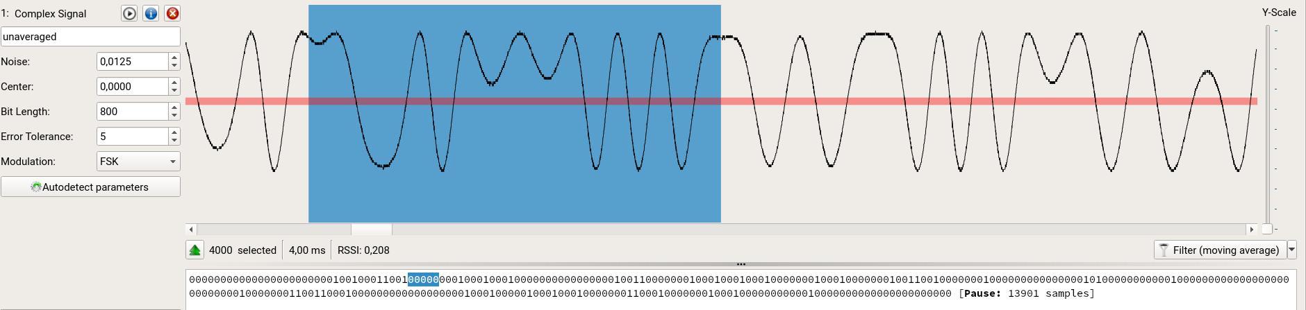
Figure 10: Signal with quantization errors.

The reason for this is that there are quantization errors in the signal. This can either be fixed with better recording hardware or by clicking the filter button below the signal. This will improve demodulation results by applying a moving average filter to the signal. The filter can be fine tuned and customized using the little arrow on the right of the button and choosing Configure filter.... This opens the filter configuration dialog.

4 Analysis

In Interpretation phase, we demodulated a signal and transformed the sine waves into bits. But what do these bits mean? To find out, we need to perform protocol reverse engineering. URH supports this process with the Analysis tab (fig. 11). We will break down the various features of this tab in this section.

Figure 11: Analysis tab.

4.1 Getting data into analysis

Before we explore this tab in more detail, let’s see how you can get data into the Analysis tab. There are three ways:

From Interpretation tab: This is the default way. The bits from each signal you open in Interpretation tab will automatically be added to Analysis tab.
Load a .proto file: With the save button in the top right of the Analysis tab, you can save your protocol and load it again via File→Open.
Load plain bits from .txt file: Got some bits lying around you want to make a quick analysis for? Just save your bits into a file that ends with .txt and open it via File→Open. Make sure your file only contains characters 1 and 0. This is also useful when your bits come from an external application.

4.2 Project files

A word of caution here: You already made some adjustments in the Interpretation tab and will probably do a lot more in Analysis tab. Your work will be lost when you close the program unless you create a project. You can convert your current work to a project any time via File→New Project. This will give you a dialog (fig. 12) for your new project.

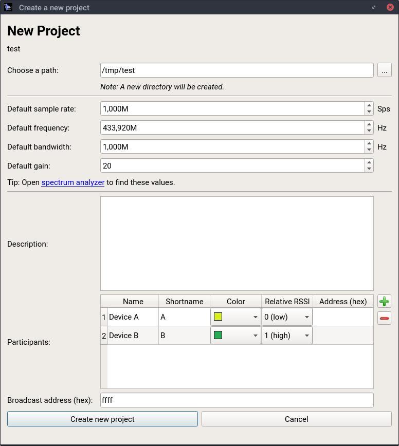
Figure 12: Dialog for creating a new project. All your changes from a non-project will be transferred to the new project.

All you need to do is to choose a directory where your project shall be saved to. Furthermore, you can make some default settings for your project and add a description. You can also configure the participants (see section 4.5), such as a remote control or a smart home central that are investigated in this project. Although you create a new project, your current work will be transferred, given that you are not already working on a project. If you want to make a fresh start, just close everything before creating a new project via File→Close all.

4.3 View data from different perspectives

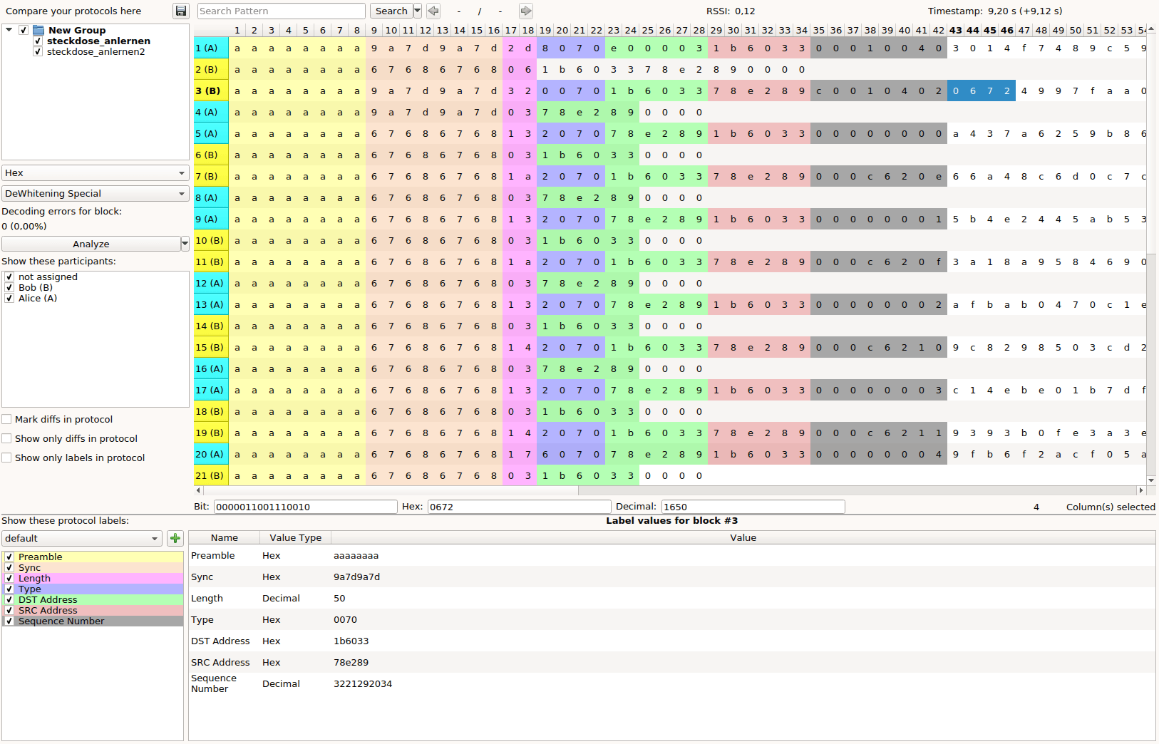
Let’s start exploring the Analysis tab by looking at the top of it first as shown in fig. 13.

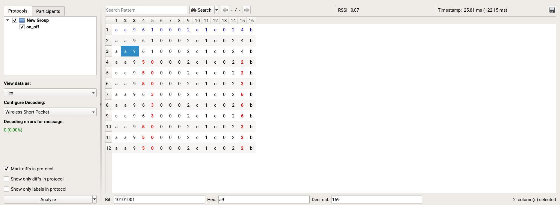
Figure 13: Top part of the Analysis tab.

All messages are aligned under each other in the center table for easy comparison. For convenience, you can mark differences using the checkbox at the bottom left of fig. 13.

The top row above the table allows you to:

Search for patterns in the data.
View the Received Signal Strength Indicator, RSSI, of the selected message.
View the absolute and relative timestamp for the selected message.
Save the current protocol with the button on the right.

Right below the table, you see current selection in Bit, Hex and Decimal representation.

Now, let’s have a look at the left part of fig. 13. In the Protocols tab, you can define which protocols you want to see in the table. Simply uncheck a protocol to hide it. For a better structure, you can also create groups using the context menu and move your protocols around these groups using drag and drop or using the context menu. In the participants tab, you can hide messages from certain participants (see section 4.5).

With the View data as combobox you can choose how the data in the table should be presented: Bit, Hex and ASCII view are supported. When opening the program, the view will default to the value set in Edit→Options→View Default View.

With the Configure decoding combobox, you can assign a decoding to the currently selected messages. You will learn more about decodings in section 4.4. Below this combobox you see how many errors occurred during decoding the selected message.

The Analyze button at the bottom le ft of fig. 13 automates many Analysis steps. It can:

Assign participants based on the RSSI of each message.
Assign decodings based on the decoding errors for each message.

Assign message types based on the configured rules described in section 4.7.
Assign labels based on heuristics for protocol labels.

You can configure Analysis button behavior using the arrow on its right. Especially when assigning different participants to many messages, this button becomes useful.

4.4 Decoding

Wireless protocols may use sophisticated encodings to prevent transmission errors or increase their energy efficiency. While this is a great idea for designing good IoT protocols, it somehow hinders you from investigating the (true) transmitted data.

4.4.1 Configure Decodings

Therefore, URH comes with a powerful decoding component. You can access it via Edit→Decoding from the main menu or by selecting ... as decoding in the Analysis tab. This will open the decoding dialog shown in fig. 14.

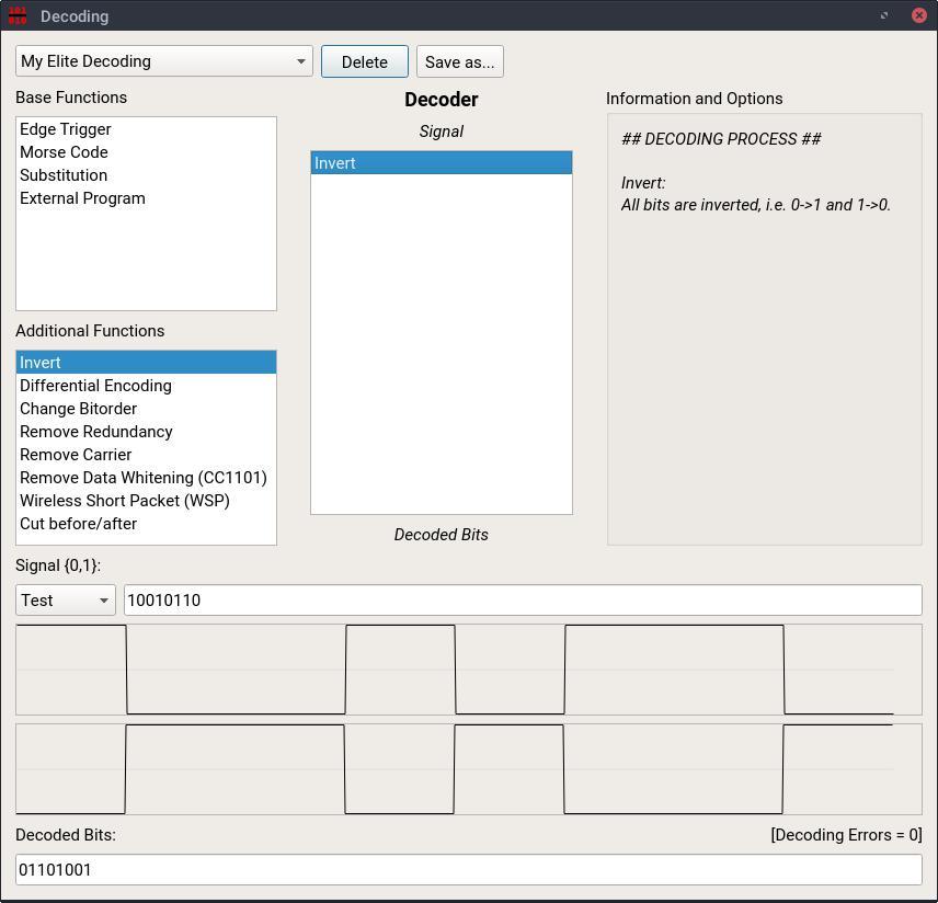
Figure 14: In the decoding dialog custom decodings can be crafted.

A decoding consists of (at least one) primitives that are chained together and processed based on their position in the list from top to bottom. You can add primitives by drag&drop.

You can preview the effect of your decoding with the fields in the lower area of the dialog. This way you can make experiments without leaving the dialog.

4.4.2 External Decodings

Have a very tough encoding and can’t find a way to build it with the given primitives? No worries! You can program your decoding in your favored language and use it right in URH!

The interface for your external program is simple:

Read the input as string (e.g., 11000) as command line argument
Write the result to STDOUT

You can learn more about external decodings in our GitHub wiki: https://github.com/jopohl/urh/wiki/Decodings#use-external-program.

4.4.3 Choose decoding

Save your new decoding with the Save as... button and it will be added to the list of available encodings in the Analysis tab. To apply your crafted decoding to your data, just select the messages you want to set it for (for all) and use the Configure Decoding combobox in the Analysis tab.

4.5 Participants

Protocol reverse engineering gets really complicated when multiple participants are involved. For example, a wireless socket may be switched from a smart home central that is triggered by a remote control. To keep an overview, URH offers configurable participants. To use this feature, you need to create or load a project (section 4.2) and configure your participants via File→Project settings. Here, you will find the table from fig. 15.

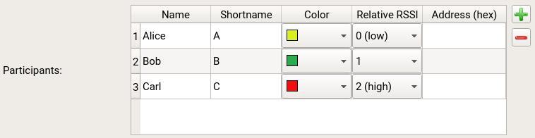
Figure 15: Use this table in project settings to configure participants.

Use the and buttons right to the table to add or remove participants, respectively. You can configure name, shortname and color of a participant to adapt it to your project. The relative RSSI will be used from URH to assign participants automatically when pressing the Analyze button (section 4.3). If you know the address of a participant, you can enter it here to help URH during automatic finding of labels when pressing the Analyze button.

To assign participants, you can either use Analyze button to do this automatically or use the context menu of the message table as shown in fig. 16.

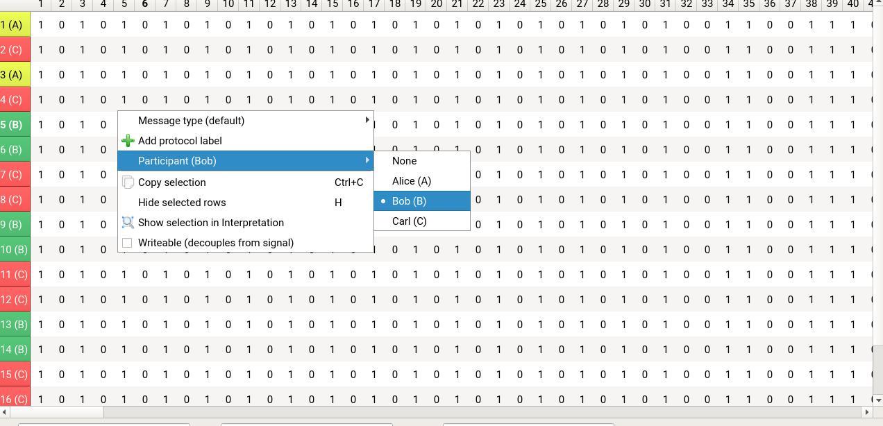
Figure 16: Manually assign a participant to selected messages with context menu.

As shown in fig. 16, each row header gets the background color of the assigned participant of the respective message. Furthermore, the participant’s shortname is added behind the row number.

With the context menu, you can also show the current selection in Interpretation. This tight integration with Interpretation allows you to find bit errors easily. Furthermore, the messages in Interpretation are also colored according to the assigned participants as shown in fig. 17.

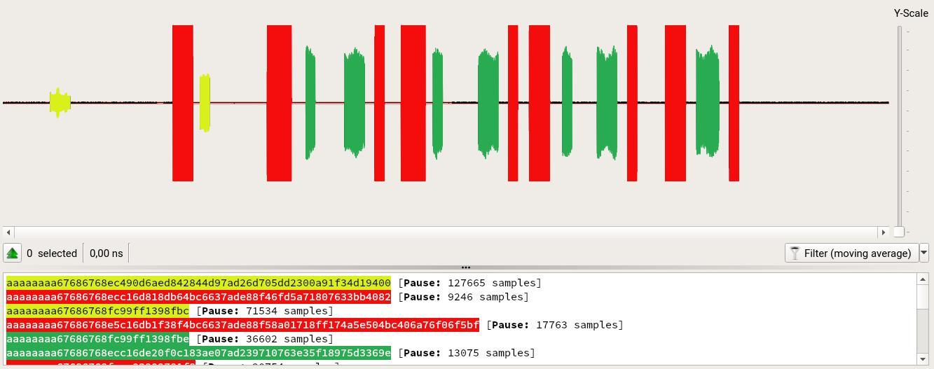
Figure 17: Participants are also visualized in Interpretation.

4.6 Labels

Messages of a protocol contain fields like Length, Address or Synchronization. During Analysis, you will reveal protocol fields one by one. To help you with this task, URH supports assigning labels to arbitrary parts of messages. These labels represent your current hypothesis for a field. You will learn how to master labels in this section.

4.6.1 Assigning and editing labels

To assign a label, simply select your desired range in message table and use context menu (right click)→Add protocol label. After adding a label, you can enter a name for it in the list view on the list view in bottom file (see fig. 18) or choose a predefined name based on the configured field types (section 4.6.2).

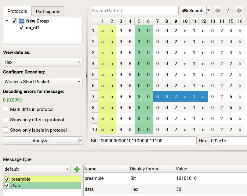
Figure 18: Assigned labels will be added to label list view and Wireshark-like preview.

Once the label is added, you notice three changes on Analysis tab:

The according data in message table is colored in label color.
The label is added to the label list on bottom left. You can also uncheck a label here to hide all ranges with this label from message table.
When moving the selection in message table, you see the values of all labels for the current message in a Wireshark-like table view below the message table. You can configure the Display format here using the combobox in the second column. Possible values are Bit, Hex, ASCII and Decimal.

In order to edit a label, simply right click on it either in message table or label list. This will open a new dialog, where you can edit name, start, end and color of each label.

4.6.2 Field Types

Field types can speed up the assigning of labels even further by defining default values for label names. Field type configuration dialog can be opened either via context menu of label list view or Edit→Options→Fieldtypes. By default, the field types from fig. 19 are available.

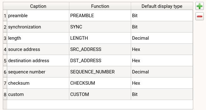
Figure 19: Configure the field types you want to use.

You can add or remove field types with the buttons right to the table. All Captions will be available when adding new labels in Analysis and also considered in autocompletion when entering a label name. This way, you can spare yourself from typing the same label names again and again for each new project.

The Default display type is the initial option for the Display format of the label preview table (bottom of fig. 18) when a new label with this field type is added.

The Function of a field type is mostly used internally by URH when it assigns labels automatically. The CHECKSUM function, however, is an exception, because it unlocks advanced functionality. Let’s explore this feature in the next section.

4.6.3 Checksum labels

If your protocol has checksums, URH can verify these for you. Simply assign a label with a field type that has CHECKSUM function configured and you will get instant feedback if the message’s checksum matches the expectation in the label preview table as shown in fig. 20.

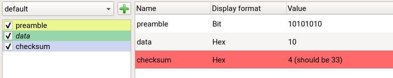
Figure 20: Feedback about checksum.

You can configure the type of the checksum in the label detail dialog. This dialog can be opened using context menu of the label in label list view or message table. Whenever a checksum label is present in the set of labels, the checksum configuration as shown in fig. 21 will appear. Here you can define a CRC polynomial (generic category) or choose the Wireless Short Packet (WSP) checksum which is included by default.

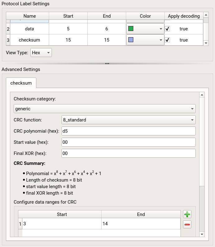
Figure 21: Checksum configuration.

In the generic category, you will always see a preview of your configured CRC so you have instant feedback when editing it. In the table at the bottom, you define for which ranges of the message the checksum shall be calculated. By default, these ranges exclude labels of type PREAMBLE and SYNC. Note, you can also add multiple ranges using the button when you have a more complicated checksum that excludes certain ranges.

4.7 Message Types

Message types take the label concept to the next level. Complex protocols tend to have different message types like ACK and DATA. By default, URH uses only one message type and applies configured labels to all messages based on their position only. With message types, you gain another level of control as you can configure labels per message type.

Message types can be added with the button next to the message type combobox right above the label list view. New message types will be bootstrapped with the labels from the default message type. You can assign message types to messages by selecting them in message table and use the context menu. This way, you can handle complex protocols like the one shown in fig. 11.

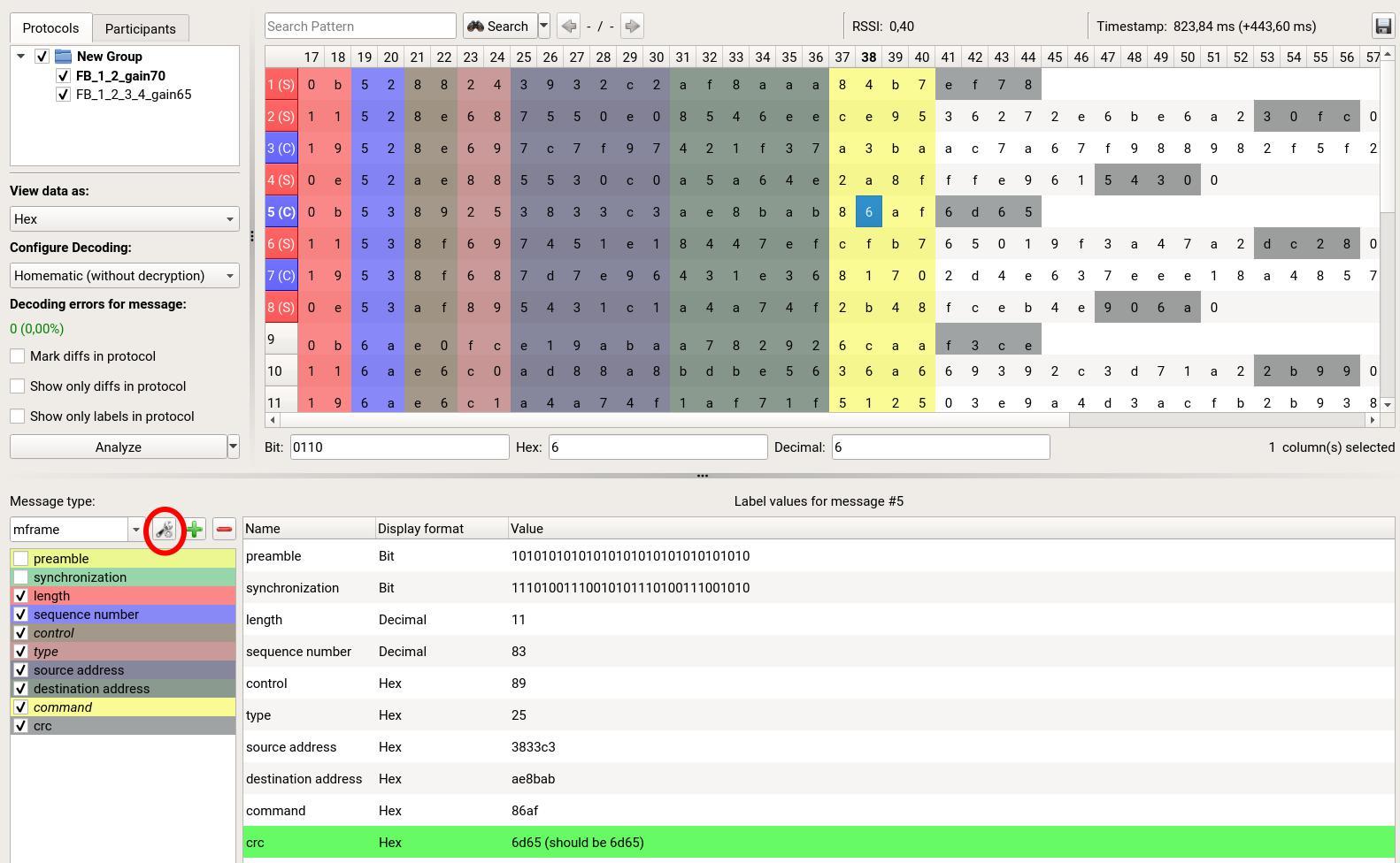
Figure 22: A more complex protocol with various message types.

Assigning message types manually can be tedious. Therefore, URH has a feature to assign message types automatically based on rules. You can configure these rules for a message type by clicking the highlighted button in fig. 22. This will pop up the rule configuration dialog. Configuring rules is straightforward using the shown table.

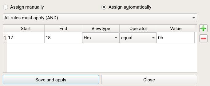
Figure 23: Rules for automatic message type assignment can be configured in this dialog.

When hitting the Save and apply button, URH will close the dialog and apply the message types based on the rules. You can also enforce the update of automatically assigned message types using the context menu of the label list view.

5 Generation

So far we have demodulated wireless signals in Interpretation and reverse engineered protocol logic in Analysis. It is time to get the reward for this work and finally break a wireless protocol. This is exactly what the Generator tab (fig. 24) is for.

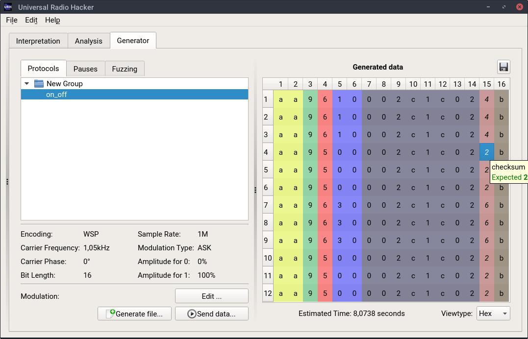
Figure 24: Generator tab.

You can add a protocol via drag&drop from the tree view on the right. As you see, all your labels from Analysis are transferred when doing this. The table is editable so you can manipulate the data. Furthermore, you can add columns or empty messages using the context menu of the table.

The Generator has also a special feature for checksum labels: It will automatically recalculate the checksum whenever you change message data. This way, you do not need to worry about the checksums when manipulating data. Moreover, a checksum label’s tooltip identifies whether the checksum is correct or not.

5.1 Fuzzing

While it is possible to edit messages by hand, it is much faster to let URH do the dirty work for us. This is the purpose of the fuzzing component. You can enter a range of values for a label you want to fuzz and just hit a button while URH takes care of the rest. Let’s see how this works.

Start by selecting your desired label in message table, then right click on it and choose Edit→fuzzing label. This will open the fuzzing dialog from fig. 25

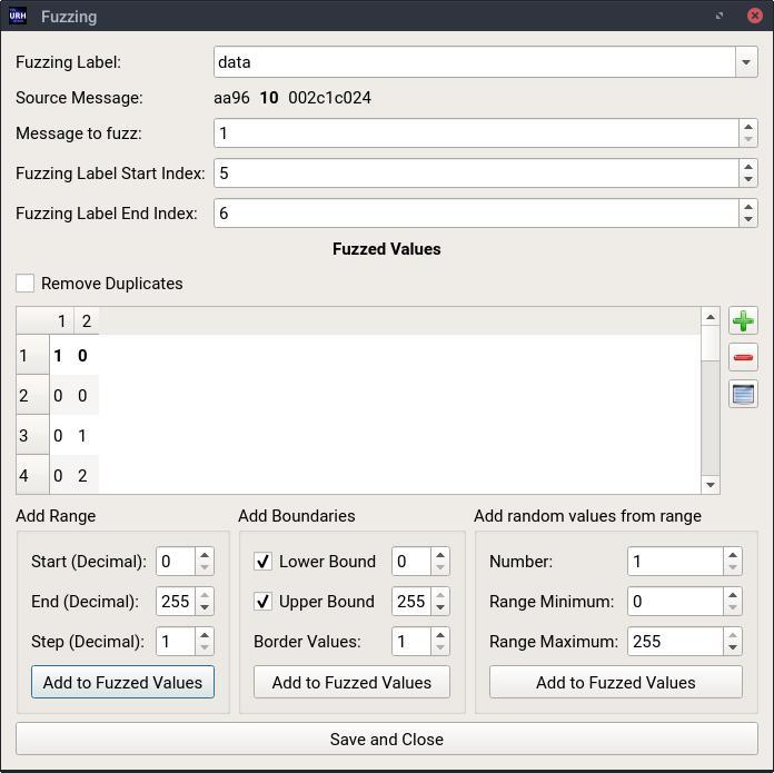
Figure 25: With the fuzzing dialog, you can quickly add value ranges for labels.

In this example, we fuzz the label data. The bold 10 indicates the original value for this message. In the center table, you define which values should be set for this label during fuzzing. With the buttons to the right of the table, you can add values manually(), or remove () and repeat () selected values, respectively.

The controls at the bottom allow you to automate the adding of values in the following ways:

Add a full range of values from Start to End, e.g. 0...255.
Add boundaries only, e.g. {0, 1, 254, 255} for Start = 0 End = 255, Border Values = 2.
Add random values from speci ed range.

When you are done, hit the Save and Close button and go to the Fuzzing tab in Generator as shown in fig. 26. Note, you configure the fuzzing settings per message so make sure you select the message you want to fuzz before making fuzzing settings. You see the number of fuzzing values behind the label name, in this case 256. Make sure you check the label you want to fuzz to activate it.

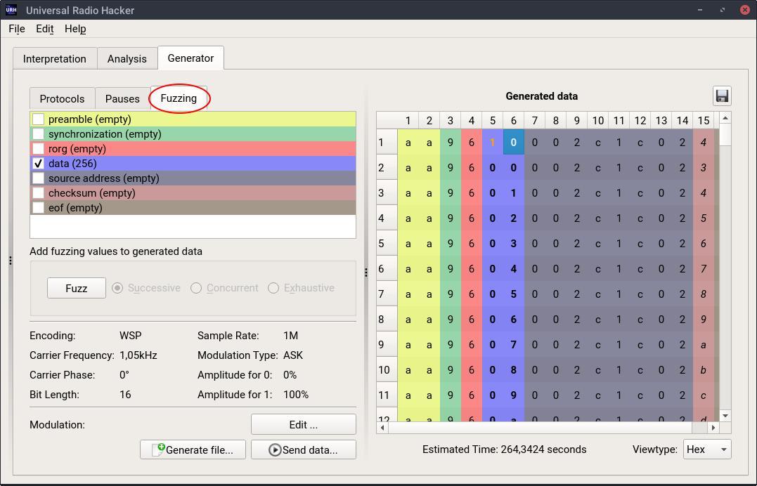
Figure 26: Fuzzing is as easy as clicking a button.

An active fuzzing label will be marked orange in the Generator table. Now everything is set up, just hit the Fuzz button and watch how URH generates all the messages. As can be seen from fig. 26it also takes care of recalculating the checksum for each fuzzed message.

By default, URH adds a pause of one mega sample before each fuzzed message. You can change this via Options Generation. Pauses between messages are itself configurable in the Pauses tab left to Fuzzing tab.

In case you want to fuzz different ranges within the same message, use the radio buttons next to the Fuzz button to select a mode to control how the values should be added:

Successive: Fuzzed values are inserted one-by-one.
Concurrent: Labels are fuzzed at the same time.
Exhaustive: Fuzzed values are inserted in all possible combinations.

Note, you can save the current fuzzing profile with the save button at the top right corner.

5.2 Modulation

Now we have manipulated the data and can send it back to the air, right? Almost! It may be necessary to fine tune the modulation first. You can do this with the Edit button to the left of the generator table. Whenever you drop a protocol to Generator, URH will automatically determine reasonable modulation settings. Complicated modulations, however, may need some manual fine-tuning. The modulation dialog (fig. 27) that opens after clicking the Edit button helps you with this.

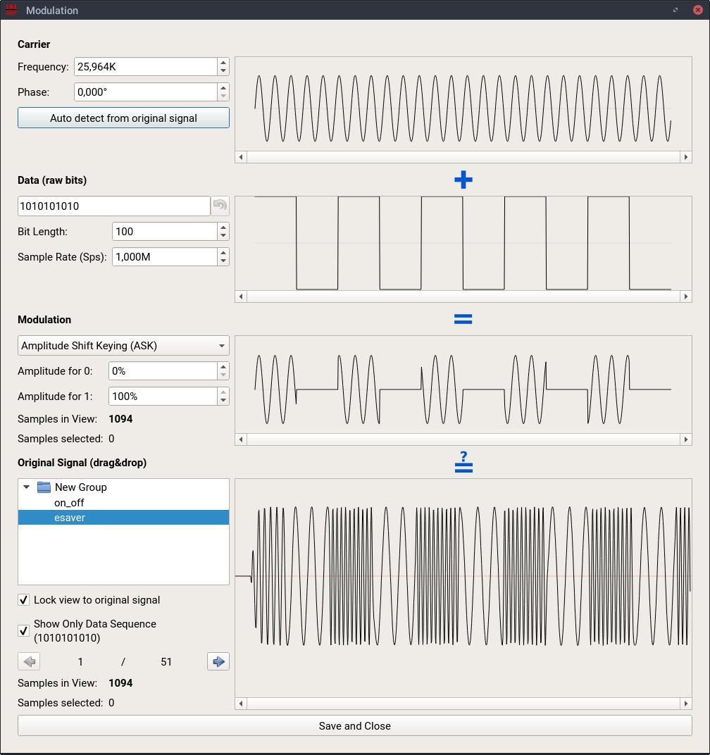
Figure 27: Fine-tune the modulation in the modulation dialog.

Simply verify all settings from top to bottom in this dialog. Each time you make a change, the modulated preview will change. You can add an original signal via drag&drop from the tree view on the bottom and use the comboboxes to only show certain ranges that represent the customizable Data (raw bits). This way, you can visually verify your modulation settings by comparing the modulation result to the original signal.

You can review modulation settings in the area left of the generator table (see fig. 26) so you do not need to open modulation dialog for this.

Note, URH automatically applies the decoding chain (section 4.4) in reverted order before modulating the data, so you do not need to bother with encoding at this stage.

5.3 Sending it back

Having made all necessary configurations, it is time to generate data. URH will take care of applying the encoding and modulating the bits. You can either use Generate left button to save this to a .complex file or hit the Send data button to open the send dialog (fig. 28).

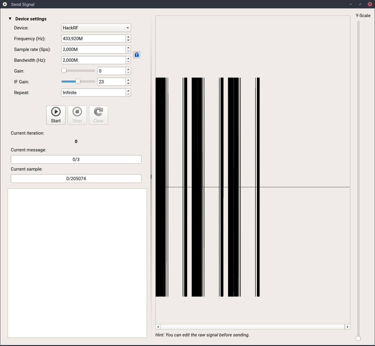
Figure 28: The send dialog will use the configured SDR to send out the data.

You see the modulated data on the right of the dialog. You can also edit the signal before sending using the context menu, if required. On the left side, SDR related settings can be made. As soon as you hit the start button, send progress will be visualized in three ways. First, you see the current message in the progress bar on the right. Second, right below this, the current sample is shown. Third, in the graphic view on the right, an indicator will be drawn and updated during sending.

Could you trigger an action on the target device? Welcome to the circle of IoT hackers!

6 Configuring Look and Feel

URH gives you a native look and feel regardless if you install it on Linux, Windows or OSX. However, if you would like to customize it, there are two fallback themes available. Figure 29 gives you an impression of how the three themes compare to each other on Windows.

(a) Native theme on Windows.

(b) Light theme. (c) Dark theme.

Figure 29: URH in the three different themes on Windows.

You can configure the theme using Edit→Options→View→Choose application theme. Linux users can also configure icon theme. This allows using system icons instead of the bundled icon theme that come with URH. You can choose this via Edit→Options→View→Choose icon theme.

Note to KDE users: If you experience icon issues in file dialogs, it is necessary to switch the icon theme to native icon theme using Edit→Options→View→Choose icon theme.

7 Plugins

URH can be enhanced using plugins. To activate a plugin, simply check its checkbox using Edit→ Options→Plugins. In this section, you will find an overview of available plugins.

ZeroHide: This plugin allows you to entirely crop long sequences of zeros in your protocol and focus on relevant data. You can set a threshold below. All sequences of directly following zeros, which are longer than this threshold, will be removed. This will give you a new entry in Analysis message table context menu.
RfCat: With this plugin, we support sending bytestreams via RfCat (e.g. using YARD Stick One). Therefore, a new button below generator table will be created.
InsertSine: This plugin enables you to insert custom sine waves into your signal as shown in fig. 30. You will find a new context menu entry in Interpretation signal view. Transform URH into a full fledged signal editor!
NetworkSDRInterface: With this plugin, you can interface external applications using TCP. You can use your external application for performing protocol simulation on logical level or advanced modulation/decoding. If you activate this plugin, a new SDR will be selectable in device dialogs. Furthermore, a new button below generator table will be created.
MessageBreak: This plugin enables you to break a protocol message on an arbitrary position. This is helpful when you have redundancy in your messages. This will give you a new entry in Analysis message table context menu.

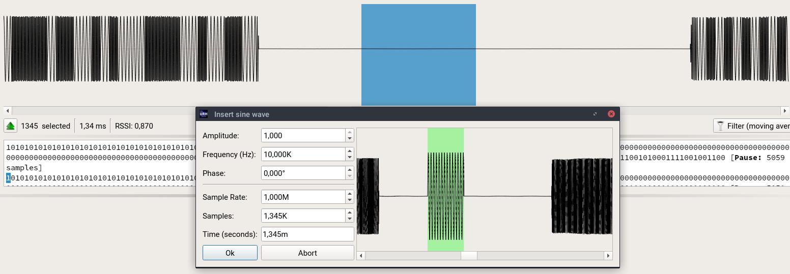
Figure 30: Insert arbitrary sine waves in Interpretation with the InsertSine plugin.

Did you liked the article? If you want to read more similar tutorials check the full free edition Open Source Tools

September 18, 2019

0 Comments

Inline Feedbacks

View all comments